Scatter itechguides labels
Table of Contents
Table of Contents
If you work with data, you’ve probably heard the term “scatter graph” or “scatter plot.” Scatter graphs are an essential tool used to display relationships between two variables. In this blog post, we’ll cover how to draw a scatter graph in excel, step by step.
Creating scatter graphs in Excel can be challenging if you’ve never done it before. The process of plotting data points, formatting axes, and adding trendlines is not always intuitive. Frustration with these steps can lead to wasted time and errors in your analysis.
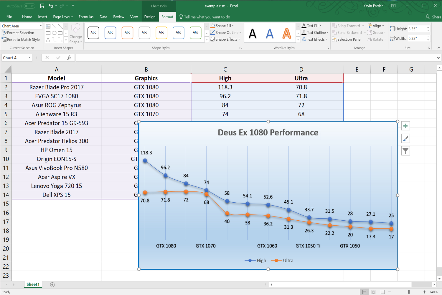
First, open a new Excel workbook and input your data into two columns. Select both columns and navigate to the “Insert” tab. Select “Scatter” from the “Charts” section. Excel will draw a basic scatter plot for you.
To customize the graph, select the graph, and navigate to the “Chart Tools” tab. Here, you can change the chart title, axes, and format the data points. To add a trendline, right-click on a data point and select “Add Trendline.” Choose the type of trendline and format it to your preference.
Overall, the process of creating a scatter graph in excel involves inputting your data, selecting a chart type, then customizing the graph to your requirements. Remember to add trendlines to identify relationships between variables accurately.
Using Excel’s Scatter Graph to Visualize Sales Data
One of my experiences using scatter graphs in excel was to visualize sales data. Sales data can provide unique insights into trends and patterns in your business, and scatter graphs can help visualize these. By plotting the data points for different products on a scatter graph, I was able to identify which products sold well together and which did not. This allowed me to make adjustments to product bundles and optimize sales.
How to Format Axis Labels and Titles
Excel has many features to customize and format your scatter graph. One of the most crucial features is the formatting of axis labels and titles. You can change the axis label from “Column A” to a descriptive title. To do so, navigate to the “Chart Tools” tab, select “Axis Titles,” and select “Primary Horizontal” or “Primary Vertical.” Here you can edit the titles for the respective axes.
How to Add Multiple Data Sets to a Scatter Graph
Adding multiple data sets to a scattergraph allows you to visualize multiple relationships between variables at once. To add multiple data sets in excel, you need to select the chart, navigate to “Chart Tools,” and select “Select Data.” Here, you can add additional series to your chart and format axis labels and titles as desired.
How to Add Data Labels to a Scatter Graph
Data labels can be helpful to provide context to your scatter graph. Excel allows you to add data labels to each data point, displaying the value of each point. To add data labels to a scatter graph, select the chart, navigate to “Chart Tools,” and select “Series,” then “Data labels.” Here, you can format the data labels to your preference.
Conclusion of How to Draw a Scatter Graph in Excel:
Scatter graphs in Excel are an essential tool for visualizing relationships between variable data. Despite the challenges presented, creating scatter graphs in excel can be straightforward. To create a scatter graph in excel, input your data, select a chart type, and customize the graph to your requirements, adding trendlines to display relationships accurately. Using scatter graphs in excel to visualize sales data or other complex data sets, formatting axis labels and titles, adding multiple data sets and data labels can provide new insights and uncover patterns or trends in your data. Remember to follow these steps and tips to create accurate and visually appealing scatter graphs in Excel.
Question and Answer:
1. How do I customize the appearance of data points in the scatter graph?
Excel provides a variety of options for customizing data points in scatter graphs. You can change the size, color, and shape of data points by selecting a data point, right-clicking, and selecting “Format Data Point.”
2. Can I add error bars to my scatter graph in Excel?
Yes, error bars can be added to your scatter graph by selecting the chart, navigating to “Chart Tools,” and selecting “Error Bars.”
3. How do I change the scale of the Y axis?
You can change the scale of the Y axis by selecting the chart and right-clicking on the Y axis. Select “Format Axis” and use the options in the “Axis Options” section to adjust the scale of the axis.
4. Can I create a scatter graph with logarithmic axes in Excel?
Yes, Excel allows you to create scatter graphs with logarithmic axes. To do so, select the chart, right-click on the axis you want to modify, and select “Format Axis.” In the “Axis Options” section, select “Logarithmic Scale.”
Gallery
Course 3 Chapter 9 Scatter Plots And Data Analysis – TrendingWorld

Photo Credit by: bing.com /
How To Make A Scatter Plot In Excel Introduction You Make A Scatter

Photo Credit by: bing.com / excel scatter plot chart data line itechguides
How To Make A Scatter Plot In Excel (XY Chart) - Trump Excel
 - Trump Excel")
Photo Credit by: bing.com / scatter
Scatter Plot / Scatter Chart: Definition, Examples, Excel/TI-83/TI-89/

Photo Credit by: bing.com /
How To Make A Scatter Plot In Excel | Itechguides.com

Photo Credit by: bing.com / scatter itechguides labels